20 Empirical p-values
20.2 Hypothesis testing using probability models
As a lead into the central limit theorem and mathematical sampling distributions, we will look at a class of hypothesis testing where the null hypothesis specifies a probability model. In some cases we can get an exact answer and in others we will use simulation to get an empirical p-value. By the way, a permutation test is an exact test; by this we mean we are finding all the possible permutations in the calculation of the p-value. However, since the complete enumeration of all permutations is often difficult, we approximate it with randomization, simulation. Thus the p-value from a randomization test is an approximation of the exact test.
Let’s use three examples to illustrate the ideas of this lesson.
20.3 Tappers and listeners
Here’s a game you can try with your friends or family: pick a simple, well-known song, tap that tune on your desk, and see if the other person can guess the song. In this simple game, you are the tapper, and the other person is the listener.
A Stanford University graduate student named Elizabeth Newton conducted an experiment using the tapper-listener game.78 In her study, she recruited 120 tappers and 120 listeners into the study. About 50% of the tappers expected that the listener would be able to guess the song. Newton wondered, is 50% a reasonable expectation?
20.3.1 Step 1- State the null and alternative hypotheses
Newton’s research question can be framed into two hypotheses:
\(H_0\): The tappers are correct, and generally 50% of the time listeners are able to guess the tune. \(p = 0.50\)
\(H_A\): The tappers are incorrect, and either more than or less than 50% of listeners will be able to guess the tune. \(p \neq 0.50\)
Exercise: Is this a two-sided or one-sided hypothesis test? How many variables are in this model?
The tappers think that listeners will guess the song 50% of the time, so this is a two-sided test since we don’t know before hand if listeners will be better or worse than this value.
There is only one variable, is the listener correct?
20.3.2 Step 2 - Compute a test statistic.
In Newton’s study, only 42, (we changed the number to make this problem more interesting from an educational perspective) out of 120 listeners (\(\hat{p} = 0.35\)) were able to guess the tune! From the perspective of the null hypothesis, we might wonder, how likely is it that we would get this result from chance alone? That is, what’s the chance we would happen to see such a small fraction if \(H_0\) were true and the true correct-guess rate is 0.50?
Now before we use simulation, let’s frame this as a probability model. The random variable \(X\) is the number of correct out of 120. If the observations are independent and the probability of success is constant then we could use a binomial model. We can’t answer the validity of these assumptions without knowing more about the experiment, the subjects, and the data collection. For educational purposes, we will assume they are valid. Thus our test statistic is the number of successes in 120 trials. The observed value is 42.
20.3.3 Step 3 - Determine the p-value.
We now want to find the p-value as \(2 \cdot \mbox{P}(X \leq 42)\) where \(X\) is a binomial with \(p=0.5\) and \(n=120\). Again, the p-value is the probability of the data or more extreme given the null hypothesis is true. Here the null hypothesis being true implies that the probability of success is 0.50. We will use R to get the one-sided p-value and then double to get the p-value for the problem. We selected \(\mbox{P}(X \leq 42)\) because more extreme means the observed values and values further from the value you would get if the null hypothesis were true, which is 60 for this problem.
2*pbinom(42,120,prob=0.5)## [1] 0.001299333That is a small p-value.
20.3.4 Step 4 - Draw a conclusion
Based on our data, if the listeners were guessing correct 50% of the time, there is less than a \(0.0013\) probability that only 42 or less or 78 or more listeners would get it right. This is much less than 0.05, so we reject that the listeners are guessing correctly half of the time.
This decision region looks like the pmf in Figure 20.1, any observed values inside the red boundary lines would be consistent with the null hypothesis. Any values at the red line or more extreme would be in the rejection region. We also plotted the observed values in black.
gf_dist("binom",size=120,prob=.5,xlim=c(50,115)) %>%
  gf_vline(xintercept = c(49,71),color="red") %>%
  gf_vline(xintercept = c(42),color="black") %>%
  gf_theme(theme_bw) %>%
  gf_labs(title="Binomial pmf",subtitle="Probability of success is 0.5",y="Probability")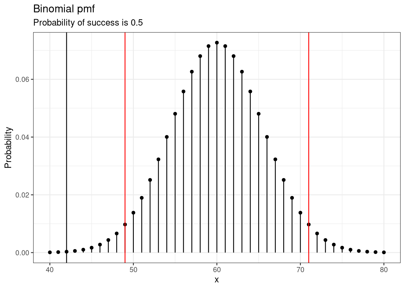
Figure 20.1: Binomial pmf
20.3.5 Repeat using simulation
We will repeat the analysis using an empirical p-value. Step 1 is the same.
20.3.6 Step 2 - Compute a test statistic.
We will use the proportion of listeners that get the song correct instead of the number, this is a minor change since we are simply dividing by 120.
obs<-42/120
obs
## [1] 0.3520.3.7 Step 3 - Determine the p-value.
To simulate 120 games under the null hypothesis where \(p = 0.50\), we could flip a coin 120 times. Each time the coin came up heads, this could represent the listener guessing correctly, and tails would represent the listener guessing incorrectly. For example, we can simulate 5 tapper-listener pairs by flipping a coin 5 times:
\[ \begin{array}{ccccc} H & H & T & H & T \\ Correct & Correct & Wrong & Correct & Wrong \\ \end{array} \]
After flipping the coin 120 times, we got 56 heads for \(\hat{p}_{sim} = 0.467\). As we did with the randomization technique, seeing what would happen with one simulation isn’t enough. In order to evaluate whether our originally observed proportion of 0.35 is unusual or not, we should generate more simulations. Here we’ve repeated this simulation 10000 times:
results <- rbinom(10000, 120, 0.5) / 120Note, we could simulate it a number of ways. Here is a way using do() that will look like how we have coded for other randomization tests.
head(results)## mean
## 1 0.4250000
## 2 0.5250000
## 3 0.5916667
## 4 0.5000000
## 5 0.5250000
## 6 0.5083333
results %>%
  gf_histogram(~mean,fill="cyan",color="black") %>%
  gf_vline(xintercept =c(obs,1-obs),color="black") %>%
  gf_theme(theme_bw()) %>%
  gf_labs(x="Test statistic")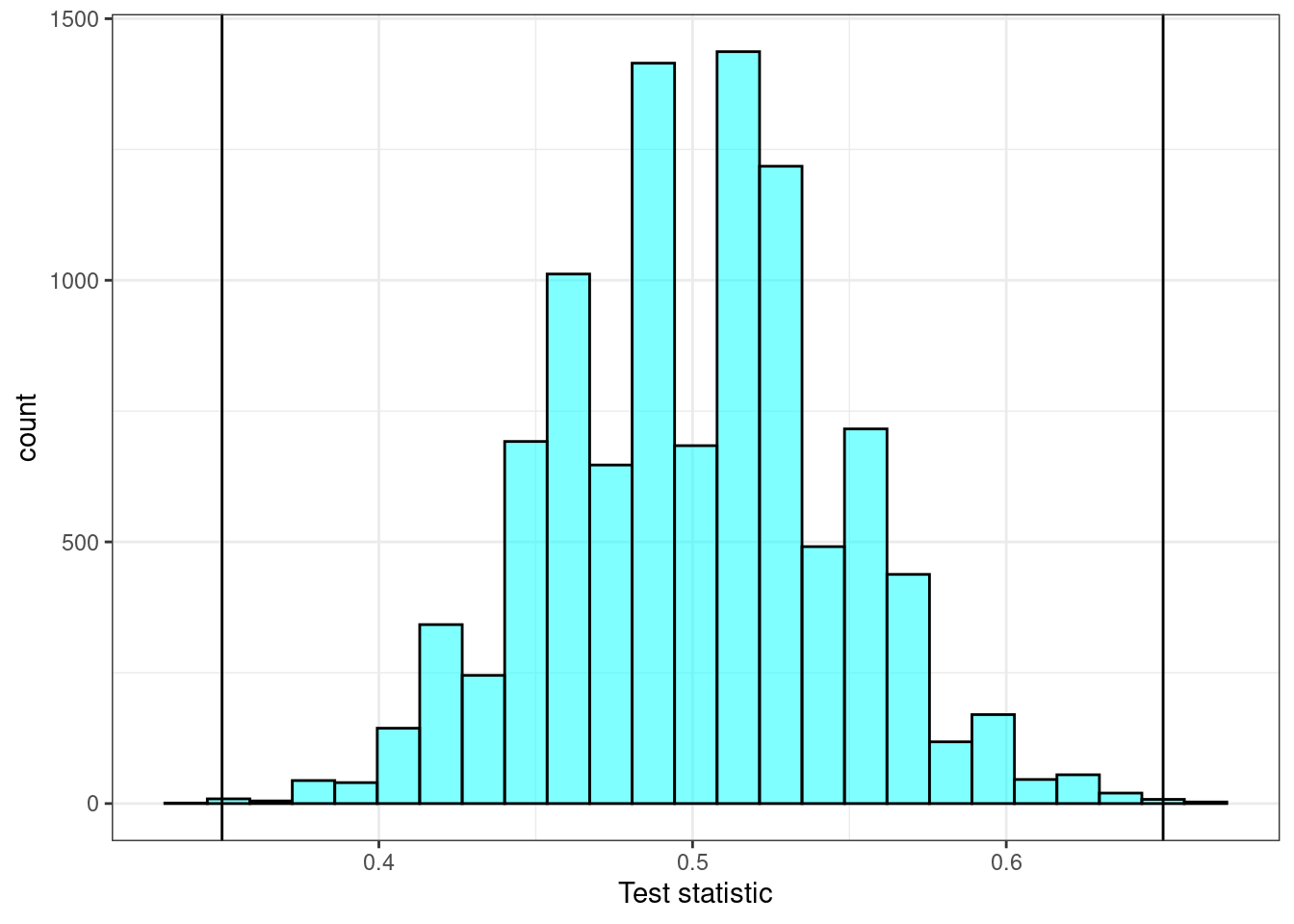
Figure 20.2: The estimated sampling distribution.
Notice in Figre 20.2 how the sampling distribution is centered at 0.5 and looks symmetrical.
The p-value is found using the prop1 function, in this problem we really need the observed case added back in to prevent a p-value of zero.
2*prop1(~(mean<=obs),data=results)## prop_TRUE
## 0.0011998820.3.8 Step 4 - Draw a conclusion
In these 10,000 simulations, we see very few results close to 0.35. Based on our data, if the listeners were guessing correct 50% of the time, there is less than a \(0.0012\) probability that only 35% or less or 65% or more listeners would get it right. This is much less than 0.05, so we reject that the listeners are guessing correctly half of the time.
Exercise: In the context of the experiment, what is the p-value for the hypothesis test?79
Exercise:
Do the data provide statistically significant evidence against the null hypothesis? State an appropriate conclusion in the context of the research question.80
20.4 Cardiopulmonary resuscitation (CPR)
Let’s return to the CPR example from last lesson. As a reminder, we will repeat the background material.
Cardiopulmonary resuscitation (CPR) is a procedure used on individuals suffering a heart attack when other emergency resources are unavailable. This procedure is helpful in providing some blood circulation to keep a person alive, but CPR chest compressions can also cause internal injuries. Internal bleeding and other injuries that can result from CPR complicate additional treatment efforts. For instance, blood thinners may be used to help release a clot that is causing the heart attack once a patient arrives in the hospital. However, blood thinners negatively affect internal injuries.
Here we consider an experiment with patients who underwent CPR for a heart attack and were subsequently admitted to a hospital.81 Each patient was randomly assigned to either receive a blood thinner (treatment group) or not receive a blood thinner (control group). The outcome variable of interest was whether the patient survived for at least 24 hours.
20.4.1 Step 1- State the null and alternative hypotheses
We want to understand whether blood thinners are helpful or harmful. We’ll consider both of these possibilities using a two-sided hypothesis test.
\(H_0\): Blood thinners do not have an overall survival effect, experimental treatment is independent of survival rate. \(p_c - p_t = 0\).
\(H_A\): Blood thinners have an impact on survival, either positive or negative, but not zero. \(p_c - p_t \neq 0\).
thinner <- read_csv("data/blood_thinner.csv")
head(thinner)## # A tibble: 6 × 2
## group outcome
## <chr> <chr>
## 1 treatment survived
## 2 control survived
## 3 control died
## 4 control died
## 5 control died
## 6 treatment survivedLet’s put it in a table.
tally(~group+outcome,data=thinner,margins = TRUE)## outcome
## group died survived Total
## control 39 11 50
## treatment 26 14 40
## Total 65 25 9020.4.2 Step 2 - Compute a test statistic.
In this case the data is from a hypergeometric distribution, this is really a binomial from a finite population. We can calculate the p-value using this probability distribution. The random variable is the number of control patients that survived from a population of 90, where 50 are control patients and 40 are treatment patients, and where a total of 25 survived.
20.4.3 Step 3 - Determine the p-value.
In this case we want to find \(\mbox{P}(X \leq 11)\) and double it since it is a two-sided test.
2*phyper(11,50,40,25)## [1] 0.2581356Note: We could have picked the lower right cell as the reference cell. But now I want the \(\mbox{P}(X \geq 14)\) with the appropriate change in parameter values. Notice we get the same answer.
2*(1-phyper(13,40,50,25))## [1] 0.2581356We could the same thing for the other two cells.
2*phyper(26,40,50,65)## [1] 0.2581356
2*(1-phyper(38,50,40,65))## [1] 0.2581356Or R has a built in function, fisher.test(), that we could use.
fisher.test(tally(~group+outcome,data=thinner))##
## Fisher's Exact Test for Count Data
##
## data: tally(~group + outcome, data = thinner)
## p-value = 0.2366
## alternative hypothesis: true odds ratio is not equal to 1
## 95 percent confidence interval:
## 0.6794355 5.4174460
## sample estimates:
## odds ratio
## 1.895136The p-value is slightly different since the hypergeometric is not symmetric. Doubling the p-value from the single side result is not quite right. The algorithm in fisher.test() finds and adds all probabilities less than or equal to value of \(\mbox{P}(X = 11)\), see Figure 20.3. This is the correct p-value.
gf_dist("hyper",m=50,n=40,k=25) %>%
  gf_hline(yintercept = dhyper(11,50,40,25),color="red") %>%
  gf_labs(title="Hypergeometric pmf",subtitle="Red line is P(X=11)",y="Probability") %>%
  gf_theme(theme_bw())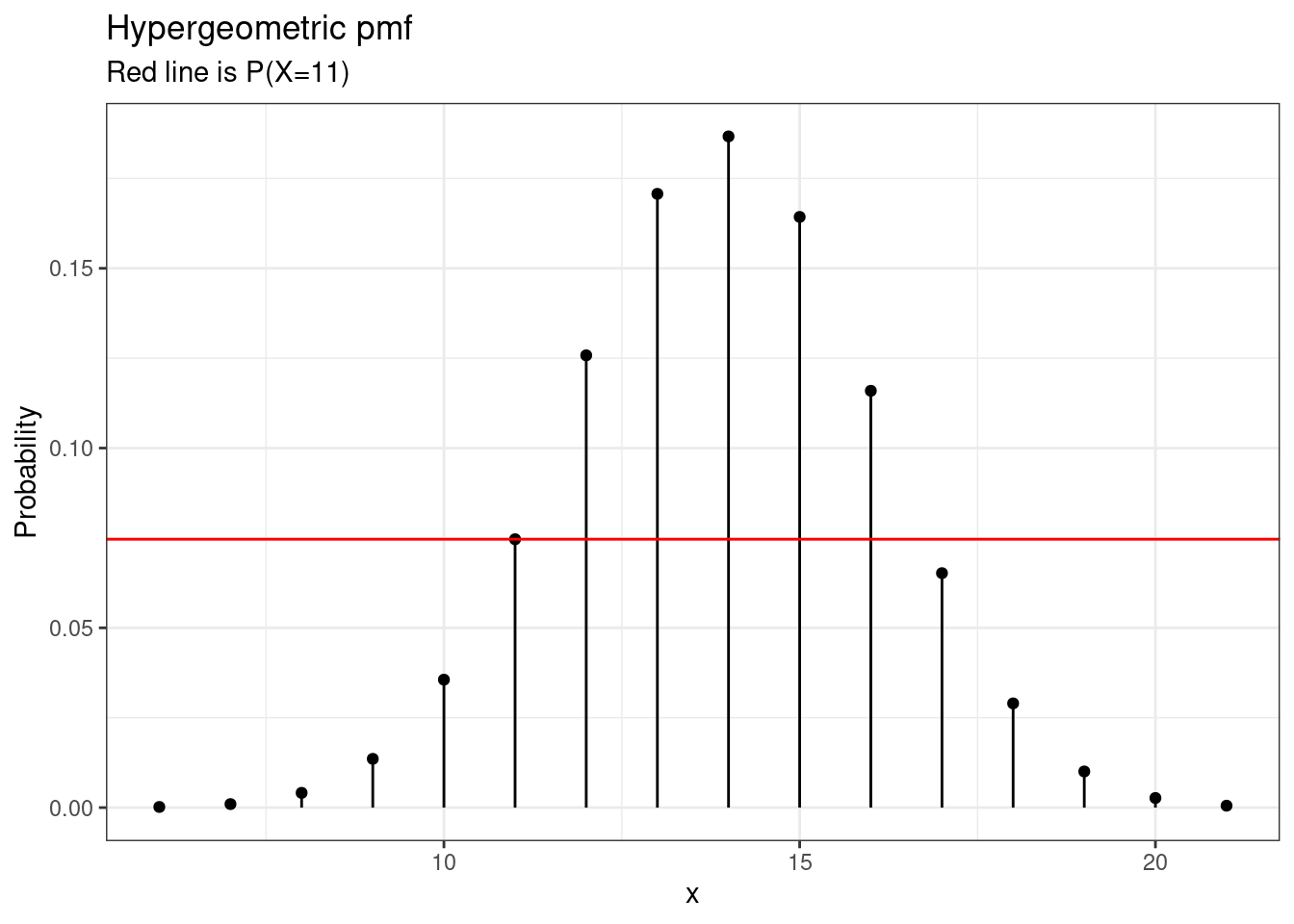
Figure 20.3: Hypergeometric pmf showing the cutoff for p-value calculation.
This is how fisher.test() is calculating the p-value:
## [1] 0.2365928The randomization test in the last lesson yielded a p-value of 0.257 so all tests are consistent.
20.4.4 Step 4 - Draw a conclusion
Since this p-value is larger than 0.05, we do not reject the null hypothesis. That is, we do not find statistically significant evidence that the blood thinner has any influence on survival of patients who undergo CPR prior to arriving at the hospital. Once again, we can discuss the causal conclusion since this is an experiment.
Notice that in these first two examples, we had a test of a single proportion and a test of two proportions. The single proportion test did not have an equivalent randomization test since there is not a second variable to shuffle. We were able to get answers since we found a probability model that we could use in each case.
20.5 Golf Balls
Our last example will be interesting because the distribution has multiple parameters and a test metric is not obvious at this point.
The owners of a residence located along a golf course collected the first 500 golf balls that landed on their property. Most golf balls are labeled with the make of the golf ball and a number, for example “Nike 1” or “Titleist 3.” The numbers are typically between 1 and 4, and the owners of the residence wondered if these numbers are equally likely (at least among golf balls used by golfers of poor enough quality that they lose them in the yards of the residences along the fairway.)
We will use a significance level of \(\alpha = 0.05\) since there is no reason to favor one error over the other.
20.5.1 Step 1- State the null and alternative hypotheses
We think that the numbers are not all equally likely. The question of one-sided versus two-sided is not relevant in this test, you will see this when we write the hypotheses.
\(H_0\): All of the numbers are equally likely.\(\pi_1 = \pi_2 = \pi_3 = \pi_4\) Or \(\pi_1 = \frac{1}{4}, \pi_2 =\frac{1}{4}, \pi_3 =\frac{1}{4}, \pi_4 =\frac{1}{4}\)
\(H_A\): There is some other distribution of percentages in the population. At least one population proportion is not \(\frac{1}{4}\).
Notice that we switched to using \(\pi\) instead of \(p\) for the population parameter. There is no reason other than to make you aware that both are used.
This problem is an extension of the binomial, instead of two outcomes, there are four outcomes. This is called a multinomial distribution. You can read more about it if you like, but our methods will not make it necessary to learn the probability mass function.
Of the 500 golf balls collected, 486 of them had a number between 1 and 4. Let’s get the data from `golf_balls.csv”.
golf_balls <- read_csv("data/golf_balls.csv")
inspect(golf_balls)##
## quantitative variables:
## name class min Q1 median Q3 max mean sd n missing
## ...1 number numeric 1 1 2 3 4 2.366255 1.107432 486 0
tally(~number,data=golf_balls)## number
## 1 2 3 4
## 137 138 107 10420.5.2 Step 2 - Compute a test statistic.
If all numbers were equally likely, we would expect to see 121.5 balls of each number, this is a point estimate and thus not an actual value that could be realized. Of course, in a sample we will have variation and thus departure from this state. We need a test statistic that will help us determine if the observed values are reasonable under the null hypothesis. Remember that the test statistics is a single number metric used to evaluate the hypothesis.
Exercise:
What would you propose for the test statistic?
With four proportions, we need a way to combine them. This seems tricky, so let’s just use a simple one. Let’s take the maximum number of balls in any cell and subtract the minimum, this is called the range and we will denote the parameter as \(R\). Under the null this should be zero. We could re-write our hypotheses as:
\(H_0\): \(R=0\)
\(H_A\): \(R>0\)
Notice that \(R\) will always be non-negative, thus this test is one-sided.
The observed range is 34, 138 - 104.
## [1] 3420.5.3 Step 3 - Determine the p-value.
We don’t know the distribution of our test statistic so we will use simulation. We will simulate data from a multinomial under the null hypothesis and calculate a new value of the test statistic. We will repeat this 10000 times and this we give us an estimate of the sampling distribution.
We will use the sample() function again to simulate the distribution of numbers under the null hypothesis. To help us understand the process and build the code, we are only initially using a sample size of 12 to keep the printout reasonable and easy to read.
## [1] 4Notice this is not using tidyverse coding ideas. We don’t think we need tibbles or data frames so we went with straight nested R code. You can break this code down by starting with the code in the center.
## [1] 3 1 2 3 2 3 1 3 3 4 1 1##
## 1 2 3 4
## 4 2 5 1## [1] 1 5## [1] 4We are now ready to ramp up to the full problem. Let’s simulated the data under the null hypothesis. We are sampling 486 golf balls with the numbers 1 through 4 on them. Each number is equally likely. We then find the range, our test statistic. Finally we repeat this 10,000 to get an estimate of the sampling distribution of our test statistic.
Figure 20.4 is a plot of the sampling distribution of the range.
results %>%
  gf_histogram(~diff,fill="cyan",color = "black") %>%
  gf_vline(xintercept = obs,color="black") %>%
  gf_labs(title="Sampling Distribution of Range",subtitle="Multinomial with equal probability",
          x="Range") %>%
  gf_theme(theme_bw)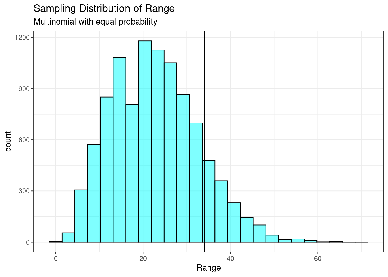
Figure 20.4: Sampling distribution of the range.
Notice how this distribution is skewed to the right.
The p-value is 0.14, this value is greater than 0.05 so we fail to reject. However, it is not that much greater than 0.05, so the residents may want to repeat the study with more data.
prop1(~(diff>=obs),data=results)## prop_TRUE
## 0.14028620.6 Repeat with a different test statistic
The test statistic we developed helped but it seems weak because we did not use the information in all four cells. So let’s devise a metric that does this. We will jump to step 2.
20.6.1 Step 2 - Compute a test statistic.
If each number were equally likely, we would have 121.5 balls in each bin. We can find a test statistic by looking at the deviation in each cell from 121.5.
tally(~number,data=golf_balls) -121.5## number
## 1 2 3 4
## 15.5 16.5 -14.5 -17.5Now we need to collapse these into a single number. Just adding will always result in a value of 0, why? So let’s take the absolute value and then add.
## [1] 64This will be our test statistic.
20.6.2 Step 3 - Determine the p-value.
We will use similar code from above with our new metric.
Figure 20.5 is a plot of the sampling distribution of the absolute value of deviations.
results %>%
  gf_histogram(~sum,fill="cyan",color="black") %>%
  gf_vline(xintercept = obs,color="black") %>%
  gf_labs(title="Sampling Distribution of Absolute Deviations",
          subtitle="Multinomial with equal probability",
          x="Absolute deviations") %>%
  gf_theme(theme_bw)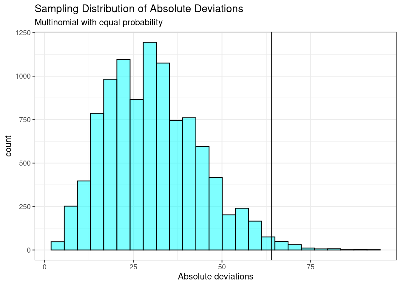
Figure 20.5: Sampling distribution of the absolute deviations.
Notice how this distribution is skewed to the right and our test statistic seems to be more extreme.
The p-value is 0.014, this value is much smaller than our previous result. The test statistic matters in our decision process as nothing about this problem has changed except the test statistic.
prop1(~(sum>=obs),data=results)## prop_TRUE
## 0.0135986420.7 Summary
In this lesson we used probability models to help us make decisions from data. This lesson is different from the randomization section in that randomization had two variables and the null hypothesis of no difference. In the case of a 2 x 2 table, we were able to show that we could use the hypergeometric distribution to get an exact p-value under the assumptions of the model.
We also found that the choice of test statistic has an impact on our decision. Even though we get valid p-values and the desired Type 1 error rate, if the information in the data is not used to its fullest, we will lose power. Note: power is the probability of rejecting the null hypothesis when the alternative hypothesis is true.
In this next lesson we will learn about mathematical solutions to finding the sampling distribution. The key difference in all these methods is the selection of the test statistic and the assumptions made to derive a sampling distribution.
20.8 Homework Problems
- Repeat the analysis of the yawning data from last lesson but this time use the hypergeometric distribution.
Is yawning contagious?
An experiment conducted by the , a science entertainment TV program on the Discovery Channel, tested if a person can be subconsciously influenced into yawning if another person near them yawns. 50 people were randomly assigned to two groups: 34 to a group where a person near them yawned (treatment) and 16 to a group where there wasn’t a person yawning near them (control). The following table shows the results of this experiment.
\[ \begin{array}{cc|ccc} & & &\textbf{Group}\\ & & \text{Treatment } & \text{Control} & \text{Total} \\ & \hline \text{Yawn} & 10 & 4 & 14 \\ \textbf{Result} & \text{Not Yawn} & 24 & 12 & 36 \\ &\text{Total} & 34 & 16 & 50 \\ \end{array} \]
The data is in the file yawn.csv.
- What are the hypotheses?
- Calculate the observed statistic, pick a cell.
- Find the p-value using the hypergeometric distribution.
- Plot the the sampling distribution.
- Determine the conclusion of the hypothesis test.
- Compare your results with the randomization test.
- Repeat the golf ball example using a different test statistic.
Use a level of significance of 0.05.
- State the null and alternative hypotheses.
- Compute a test statistic.
- Determine the p-value.
- Draw a conclusion.
- Body Temperature
Shoemaker82 cites a paper from the American Medical Association83 that questions conventional wisdom that the average body temperature of a human is 98.6. One of the main points of the original article – the traditional mean of 98.6 is, in essence, 100 years out of date. The authors cite problems with Wunderlich’s original methodology, diurnal fluctuations (up to 0.9 degrees F per day), and unreliable thermometers. The authors believe the average temperature is less than 98.6. Test the hypothesis.
- State the null and alternative hypotheses.
- State the significance level that will be used.
- Load the data from the file “temperature.csv” and generate summary statistics and a boxplot of the temperature data. We will not be using gender or heart rate for this problem.
- Compute a test statistic. We are going to help you with this part. We cannot do a randomization test since we don’t have a second variable. It would be nice to use the mean as a test statistic but we don’t yet know the sampling distribution of the sample mean.
Let’s get clever. If the distribution of the sample is symmetric, this is an assumption but look at the boxplot and summary statistics to determine if you are comfortable with it, then under the null hypothesis the observed values should be equally likely to either be greater or less than 98.6. Thus our test statistic is the number of cases that have a positive difference between the observed value and 98.6. This will be a binomial distribution with a probability of success of 0.5. You must also account for the possibility that there are observations of 98.6 in the data.
- Determine the p-value.
- Draw a conclusion.