24 Additional Hypothesis Tests
24.1 Objectives
- Conduct and interpret a hypothesis test for equality of two or more means using both permutation and the \(F\) distribution.
- Conduct and interpret a goodness of fit test using both Pearson’s chi-squared and randomization to evaluate the independence between two categorical variables.
- Conduct and interpret a hypothesis test for the equality of two variances.
- Know and check assumptions for the tests in the reading.
24.2 Introduction
The purpose of this chapter is to put all we learned in this block into perspective and then to also add a couple of new tests to demonstrate other statistical tests.
Remember that we have been using data to answer research questions. So far we can do this with hypothesis tests or confidence intervals. There is a close link between these two methods. The key ideas have been to generate a single number metric to use in answering our research question and then to obtain the sampling distribution of this metric.
In obtaining the sampling distribution we used randomization as an approximation to permutation exact tests, probability models, mathematical models, and the bootstrap. Each of these had different assumptions and different areas where they could be applied. In some cases, several methods can be applied to the problem to get a sense of the robustness to the different assumptions. For example, if you run a randomization test and a test using the CLT and they both give you similar results, you can feel better about your decision.
Finding a single number metric to answer our research question can be difficult. For example, in the homework for last chapter, we wanted to determine if the prices of books at a campus bookstore were different from Amazon’s prices. The metric we decided to use was the mean of the differences in prices. But is this the best way to answer the question? This metric has been used historically because of the need to use the \(t\) distribution. However, there are other ways in which the prices of books can differ. Jack Welch was the CEO of GE for years and he made the claim that customers don’t care about average but they do care about variability. The average temperature setting of your GE refrigerator could be off and you would adapt. However if the temperature had great variability, then you would be upset. So maybe metrics that incorporate variability might be good. In our bootstrap notes, we looked at the ages of males and females in the HELP study. In using a randomization permutation test, we assumed there was no difference in the distribution of ages between males and females. However, in the alternative we measured the difference in the distributions using only means. The means of these two populations could be equal but the distributions differ in other ways, for example variability. We could conduct a separate test for variances but we have to be careful about multiple comparisons because in that case the Type 1 error is inflated.
We also learned that the use of the information in the data impacts the power of the test. In the golf ball example, when we used range as our metric, we did not have the same power as looking at the differences from expected values under the null hypothesis. There is some mathematical theory that leads to better estimators, they are called likelihood ratio tests, but this is beyond the scope of the book. What you can do is create a simulation where you simulate data from the alternative hypothesis and then measure the power. This will give you a sense of the quality of your metric. We only briefly looked at measuring power an earlier chapter and will not go further into this idea in this chapter.
We will finish this block by examining problems with two variables. In the first case they will both be categorical but at least one of the categorical variables has more than two levels. In the second case, we will examine two variables where one is numeric and the other categorical. The categorical variable has more than two levels.
24.3 Categorical data
It is worth spending some time on common approaches to categorical data that you may come across. We have already dealt with categorical data to some extent in this course. We have performed hypothesis tests and built confidence intervals for \(\pi\), the population proportion of “success” in binary cases (for example, support for a local measure in a vote). This problem had a single variable. Also, the golf ball example involved counts of four types of golf ball. This is considered categorical data because each observation is characterized by a qualitative value (number on the ball). The data are summarized by counting how many balls in a sample belong to each type. This again was a single variable.
In another scenario, suppose we are presented with two qualitative variables and would like to know if they are independent. For example, we have discussed methods for determining whether a coin could be fair. What if we wanted to know whether flipping the coin during the day or night changes the fairness of the coin? In this case, we have two categorical variables with two levels each: result of coin flip (heads vs tails) and time of day (day vs night). We have solved this type of problem by looking at a difference in probabilities of success using randomization and mathematically derived solutions, CLT. We also used a hypergeometric distribution to obtain an exact p-value.
We will next explore a scenario that involves categorical data with two variables but where at least one variable has more than two levels. However, note that we are only merely scratching the surface in our studies. You could take an entire course on statistical methods for categorical data. This book is giving you a solid foundation to learn more advanced methods.
24.3.1 HELP example
Let’s return to Health Evaluation and Linkage to Primary Care data set, HELPrct in the mosaicData package. Previously, we looked at the differences in ages between males and females, let’s now do the same thing for the variable substance, the primary substance of abuse.
There are three substances: alcohol, cocaine, and heroin. We’d like to know if there is evidence that the proportions of use differ for men and for women. In our data set, we observe modest differences.
tally( substance ~ sex, data = HELPrct,
format="prop", margins = TRUE)
## sex
## substance female male
## alcohol 0.3364486 0.4075145
## cocaine 0.3831776 0.3208092
## heroin 0.2803738 0.2716763
## Total 1.0000000 1.0000000But we need a test statistic to test if there is a difference in substance of abuse between males and females.
24.3.2 Test statistic
To help us develop and understand a test statistic, let’s simplify and use a simple theoretical example.
Suppose we have a 2 x 2 contingency table like the one below. \[ \begin{array}{lcc} & \mbox{Response 1} & \mbox{Response 2} \\ \mbox{Group 1} & n_{11} & n_{12} \\ \mbox{Group 2} & n_{21} & n_{22} \end{array} \]
If our null hypothesis is that the two variables are independent, a classical test statistic used is the Pearson chi-squared test statistic (\(X^2\)). This is similar to the one we used in our golf ball example. Let \(e_{ij}\) be the expected count in the \(i\)th row and \(j\)th column under the null hypothesis, then the test statistic is: \[ X^2=\sum_{i=1}^2 \sum_{j=1}^2 {(n_{ij}-e_{ij})^2\over e_{ij}} \]
But how do we find \(e_{ij}\)? What do we expect the count to be under \(H_0\)? To find this, we recognize that under \(H_0\) (independence), a joint probability is equal to the product of the marginal probabilities. Let \(\pi_{ij}\) be the probability of an outcome appearing in row \(i\) and column \(j\). In the absence of any other information, our best guess at \(\pi_{ij}\) is \(\hat{\pi}_{ij}={n_{ij}\over n}\), where \(n\) is the total sample size. But under the null hypothesis we have the assumption of independence, thus \(\pi_{ij}=\pi_{i+}\pi_{+j}\) where \(\pi_{i+}\) represents the total probability of ending up in row \(i\) and \(\pi_{+j}\) represents the total probability of ending up in column \(j\). Note that \(\pi_{i+}\) is estimated by \(\hat{\pi}_{i+}\) and \[ \hat{\pi}_{i+}={n_{i+}\over n} \] Thus for our simple 2 x 2 example, we have:
\[ \hat{\pi}_{i+}={n_{i+}\over n}={n_{i1}+n_{i2}\over n} \]
And for Group 1 we would have:
\[ \hat{\pi}_{1+}={n_{1+}\over n}={n_{11}+n_{12}\over n} \]
So, under \(H_0\), our best guess for \(\pi_{ij}\) is: \[ \hat{\pi}_{ij}=\hat{\pi}_{i+}\hat{\pi}_{+j}={n_{i+}\over n}{n_{+j}\over n} = {n_{i1}+n_{i2}\over n}{n_{1j}+n_{2j}\over n} \]
Continuing, under \(H_0\) the expected cell count is:
\[ e_{ij}=n\hat{\pi}_{ij}=n{n_{i+}\over n}{n_{+j}\over n}={n_{i+}n_{+j}\over n} \]
This may look too abstract, so let’s break it down with an example, totally made up by the way.
Suppose we flip a coin 40 times during the day and 40 times at night and obtain the results below. \[ \begin{array}{lcc} & \mbox{Heads} & \mbox{Tails} \\ \mbox{Day} & 22 & 18 \\ \mbox{Night} & 17 & 23 \end{array} \]
To find the Pearson chi-squared (\(X^2\)), we need to figure out the expected value under \(H_0\). Recall that under \(H_0\) the two variables are independent. It’s helpful to add the row and column totals prior to finding expected counts:
\[ \begin{array}{lccc} & \mbox{Heads} & \mbox{Tails} & \mbox{Row Total}\\ \mbox{Day} & 22 & 18 & 40\\ \mbox{Night} & 17 & 23 & 40 \\ \mbox{Column Total} & 39 & 41 & 80 \end{array} \]
Thus under independence, expected count is equal to the row sum multiplied by the column sum divided by the overall sum. So,
\[ e_{11} = {40*39\over 80}= 19.5 \]
Continuing in this fashion yields the following table of expected counts:
\[ \begin{array}{lcc} & \mbox{Heads} & \mbox{Tails} \\ \mbox{Day} & 19.5 & 20.5 \\ \mbox{Night} & 19.5 & 20.5 \end{array} \]
Now we can find \(X^2\): \[ X^2= {(22-19.5)^2\over 19.5}+{(17-19.5)^2\over 19.5}+{(18-20.5)^2\over 20.5}+{(23-20.5)^2\over 20.5} \]
As you can probably tell, \(X^2\) is essentially comparing the observed counts with the expected counts under \(H_0\). The larger the difference between observed and expected, the larger the value of \(X^2\). It is normalized by dividing by the expected counts since more data in a cell leads to a larger contribution to the sum. Under \(H_0\), this statistic follows the chi-squared distribution with \((R-1)(C-1)\), in this case 1, degrees of freedom (\(R\) is the number of rows and \(C\) is the number of columns).
24.3.2.1 p-value
To find the Pearson chi-squared statistic (\(X^2\)) and corresponding p-value from the chi-squared distribution in R use the following code:
## [1] 1.250782
1-pchisq(x2,1)## [1] 0.2634032Note that the chi-squared test statistic is a sum of squared differences. Thus its distribution, a chi-squared, is skewed right and bounded on the left at zero. A departure from the null hypothesis means a value further in the right tail of the distribution. This is why we use one minus the CDF in the calculation of the p-value.
Again, the \(p\)-value suggests there is not enough evidence to say these two variables are dependent.
Of course there is a built in function in R that will make the calculations easier. It is chisq.test().
coin <- tibble(time = c(rep("Day",40),rep("Night",40)),
               result = c(rep(c("Heads","Tails"),c(22,18)),rep(c("Heads","Tails"),c(17,23))))
tally(~time+result,data=coin)## result
## time Heads Tails
## Day 22 18
## Night 17 23
chisq.test(tally(~time+result,data=coin),correct = FALSE)##
## Pearson's Chi-squared test
##
## data: tally(~time + result, data = coin)
## X-squared = 1.2508, df = 1, p-value = 0.2634If you just want the test statistic, which we will for permutation tests, then use:
chisq(~time+result,data=coin)## X.squared
## 1.25078224.3.3 Extension to larger tables
The advantage of using the Pearson chi-squared is that it can be extended to larger contingency tables, the name given to these tables of multiple categorical variables. Suppose we are comparing two categorical variables, one with \(r\) levels and the other with \(c\) levels. Then, \[ X^2=\sum_{i=1}^r \sum_{j=1}^c {(n_{ij}-e_{ij})^2\over e_{ij}} \]
Under the null hypothesis of independence, the \(X^2\) test statistic follows the chi-squared distribution with \((r-1)(c-1)\) degrees of freedom.
24.3.4 Permutation test
We will complete our analysis of the HELP data first using a randomization, approximate permutation, test.
First let’s write the hypotheses:
\(H_0\): The variables sex and substance are independent.
\(H_a\): The variables sex and substance are dependent.
We will use the chi-squared test statistic as our test statistic. We could use a different test statistic such as using the absolute value function instead of the square function but then we would need to write a custom function.
First, let’s get the observed value for the test statistic:
obs <- chisq(substance~sex,data=HELPrct)
obs
## X.squared
## 2.026361Next we will use a permutation randomization process to find the sampling distribution of our test statistics.
Figure 24.1 is a visual summary of the results which helps us to gain some intuition about the p-value. We also plot the theoretical chi-squared distribution as a dark blue overlay.
results %>%
  gf_dhistogram(~X.squared,fill="cyan",color="black") %>%
  gf_vline(xintercept = obs,color="red") %>%
  gf_theme(theme_classic()) %>%
  gf_dist("chisq",df=2,color="darkblue") %>%
  gf_labs(title="Sampling distribution of chi-squared test statistic",
          subtitle="For the variables sex and substance in the HELPrct data set",
          x="Test statistic")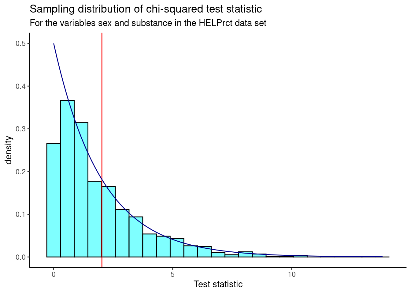
Figure 24.1: Sampling distribution of chi-squared statistic from randomization test.
We find the p-value using prop1().
prop1((~X.squared>=obs),data=results)## prop_TRUE
## 0.3536464We don’t double this value because the chi-squared is a one sided test due to the fact that we squared the differences.
Based on this p-value, we fail to reject the hypothesis that the variables are independent.
24.3.5 Chi-squared test
We will jump straight to using the function chisq.test().
chisq.test(tally(substance~sex,data=HELPrct))##
## Pearson's Chi-squared test
##
## data: tally(substance ~ sex, data = HELPrct)
## X-squared = 2.0264, df = 2, p-value = 0.3631We get a p-value very close to the one from the randomization permutation test. Remember in the randomization test we shuffled the variable sex over many replications and calculated a value for the test statistic for each replication. We did this shuffling because the null hypothesis assumed independence of the two variables. This process led to an empirical estimate of the sampling distribution, the gray histogram in the previous graph. In this section, under the null hypothesis and the appropriate assumptions, the sampling distribution is a chi-squared, the blue line in the previous graph. We used it to calculate the p-value directly.
Notice that if the null hypothesis is true the test statistic has the minimum value of zero. We can’t use a bootstrap confidence interval on this problem because zero will never be in the interval. It can only be on the edge of an interval.
24.4 Numerical data
Sometimes we want to compare means across many groups. In this case we have two variables where one is continuous and the other categorical. We might initially think to do pairwise comparisons, two sample t-tests, as a solution; for example, if there were three groups, we might be tempted to compare the first mean with the second, then with the third, and then finally compare the second and third means for a total of three comparisons. However, this strategy can be treacherous. If we have many groups and do many comparisons, it is likely that we will eventually find a difference just by chance, even if there is no difference in the populations.
In this section, we will learn a new method called analysis of variance (ANOVA) and a new test statistic called \(F\). ANOVA uses a single hypothesis test to check whether the means across many groups are equal. The hypotheses are:
\(H_0\): The mean outcome is the same across all groups. In statistical notation, \(\mu_1 = \mu_2 = \cdots = \mu_k\) where \(\mu_i\) represents the mean of the outcome for observations in category \(i\).
\(H_A\): At least one mean is different.
Generally we must check three conditions on the data before performing ANOVA with the \(F\) distribution:
- the observations are independent within and across groups,
- the data within each group are nearly normal, and
- the variability across the groups is about equal.
When these three conditions are met, we may perform an ANOVA to determine whether the data provide strong evidence against the null hypothesis that all the \(\mu_i\) are equal.
24.4.1 MLB batting performance
We would like to discern whether there are real differences between the batting performance of baseball players according to their position: outfielder (OF), infielder (IF), designated hitter (DH), and catcher (C). We will use a data set mlbbat10 from the openintro package but we saved it is in the file mlb_obp.csv which has been modified from the original data set to include only those with more than 200 at bats. The batting performance will be measured with the on-base percentage. The on-base percentage roughly represents the fraction of the time a player successfully gets on base or hits a home run.
Read the data into R.
mlb_obp <- read_csv("data/mlb_obp.csv")Let’s review our data:
inspect(mlb_obp)##
## categorical variables:
## name class levels n missing
## 1 position character 4 327 0
## distribution
## 1 IF (47.1%), OF (36.7%), C (11.9%) ...
##
## quantitative variables:
## name class min Q1 median Q3 max mean sd n
## ...1 obp numeric 0.174 0.309 0.331 0.3545 0.437 0.332159 0.03570249 327
## missing
## ...1 0Next change the variable position to a factor to give us greater control.
favstats(obp~position,data=mlb_obp)## position min Q1 median Q3 max mean sd n missing
## 1 C 0.219 0.30000 0.3180 0.35700 0.405 0.3226154 0.04513175 39 0
## 2 DH 0.287 0.31625 0.3525 0.36950 0.412 0.3477857 0.03603669 14 0
## 3 IF 0.174 0.30800 0.3270 0.35275 0.437 0.3315260 0.03709504 154 0
## 4 OF 0.265 0.31475 0.3345 0.35300 0.411 0.3342500 0.02944394 120 0The means for each group are pretty close to each other.
Exercise: The null hypothesis under consideration is the following: \(\mu_{OF} = \mu_{IF} = \mu_{DH} = \mu_{C}\). Write the null and corresponding alternative hypotheses in plain language.89
If we have all the data for the 2010 season, why do we need a hypothesis test? What is the population of interest?
If we are only making decisions or claims about the 2010 season, we do not need hypothesis testing. We can just use summary statistics. However, if we want to generalize to other years or other leagues, then we would need a hypothesis test.
Exercise:
Construct side-by-side boxplots.
Figure 24.2 is the side-by-side boxplots.
mlb_obp %>%
  gf_boxplot(obp~position) %>%
  gf_labs(x="Position Played",y="On Base Percentage") %>%
  gf_theme(theme_bw()) %>%
  gf_labs(title="Comparison of OBP for different positions")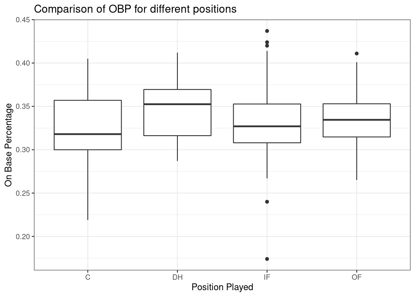
Figure 24.2: Boxplots of on base percentage by position played.
The largest difference between the sample means is between the designated hitter and the catcher positions. Consider again the original hypotheses:
\(H_0\): \(\mu_{OF} = \mu_{IF} = \mu_{DH} = \mu_{C}\)
\(H_A\): The average on-base percentage (\(\mu_i\)) varies across some (or all) groups.
Why might it be inappropriate to run the test by simply estimating whether the difference of \(\mu_{DH}\) and \(\mu_{C}\) is statistically significant at a 0.05 significance level? The primary issue here is that we are inspecting the data before picking the groups that will be compared. It is inappropriate to examine all data by eye (informal testing) and only afterwards decide which parts to formally test. This is called data snooping or data fishing. Naturally we would pick the groups with the large differences for the formal test, leading to an inflation in the Type 1 Error rate. To understand this better, let’s consider a slightly different problem.
Suppose we are to measure the aptitude for students in 20 classes in a large elementary school at the beginning of the year. In this school, all students are randomly assigned to classrooms, so any differences we observe between the classes at the start of the year are completely due to chance. However, with so many groups, we will probably observe a few groups that look rather different from each other. If we select only these classes that look so different, we will probably make the wrong conclusion that the assignment wasn’t random. While we might only formally test differences for a few pairs of classes, we informally evaluated the other classes by eye before choosing the most extreme cases for a comparison.
In the next section we will learn how to use the \(F\) statistic and ANOVA to test whether observed differences in means could have happened just by chance even if there was no difference in the respective population means.
24.4.2 Analysis of variance (ANOVA) and the F test
The method of analysis of variance in this context focuses on answering one question: is the variability in the sample means so large that it seems unlikely to be from chance alone? This question is different from earlier testing procedures since we will simultaneously consider many groups, and evaluate whether their sample means differ more than we would expect from natural variation. We call this variability the mean square between groups (\(MSG\)), and it has an associated degrees of freedom, \(df_{G}=k-1\) when there are \(k\) groups. The \(MSG\) can be thought of as a scaled variance formula for means. If the null hypothesis is true, any variation in the sample means is due to chance and shouldn’t be too large. We typically use software to find \(MSG\), however, the derivation follows. Let \(\bar{x}\) represent the mean of outcomes across all groups. Then the mean square between groups is computed as
\[
MSG = \frac{1}{df_{G}}SSG = \frac{1}{k-1}\sum_{i=1}^{k} n_{i}\left(\bar{x}_{i} - \bar{x}\right)^2
\]
where \(SSG\) is called the sum of squares between groups and \(n_{i}\) is the sample size of group \(i\).
The mean square between the groups is, on its own, quite useless in a hypothesis test. We need a benchmark value for how much variability should be expected among the sample means if the null hypothesis is true. To this end, we compute a pooled variance estimate, often abbreviated as the mean square error (\(MSE\)), which has an associated degrees of freedom value \(df_E=n-k\). It is helpful to think of \(MSE\) as a measure of the variability within the groups. To find \(MSE\), let \(\bar{x}\) represent the mean of outcomes across all groups. Then the sum of squares total (\(SST\))} is computed as \(SST = \sum_{i=1}^{n} \left(x_{i} - \bar{x}\right)^2\), where the sum is over all observations in the data set. Then we compute the sum of squared errors (\(SSE\)) in one of two equivalent ways:
\[ SSE = SST - SSG = (n_1-1)s_1^2 + (n_2-1)s_2^2 + \cdots + (n_k-1)s_k^2 \]
where \(s_i^2\) is the sample variance (square of the standard deviation) of the residuals in group \(i\). Then the \(MSE\) is the standardized form of \(SSE\): \(MSE = \frac{1}{df_{E}}SSE\).
When the null hypothesis is true, any differences among the sample means are only due to chance, and the \(MSG\) and \(MSE\) should be about equal. As a test statistic for ANOVA, we examine the fraction of \(MSG\) and \(MSE\):
\[F = \frac{MSG}{MSE}\]
The \(MSG\) represents a measure of the between-group variability, and \(MSE\) measures the variability within each of the groups. Using a permutation test, we could look at the difference in the mean squared errors as a test statistic instead of the ratio.
We can use the \(F\) statistic to evaluate the hypotheses in what is called an F test. A p-value can be computed from the \(F\) statistic using an \(F\) distribution, which has two associated parameters: \(df_{1}\) and \(df_{2}\). For the \(F\) statistic in ANOVA, \(df_{1} = df_{G}\) and \(df_{2}= df_{E}\). The \(F\) is really a ratio of chi-squared distributions.
The larger the observed variability in the sample means (\(MSG\)) relative to the within-group observations (\(MSE\)), the larger \(F\) will be and the stronger the evidence against the null hypothesis. Because larger values of \(F\) represent stronger evidence against the null hypothesis, we use the upper tail of the distribution to compute a p-value.
The \(F\) statistic and the \(F\) test
Analysis of variance (ANOVA) is used to test whether the mean outcome differs across 2 or more groups. ANOVA uses a test statistic \(F\), which represents a standardized ratio of variability in the sample means relative to the variability within the groups. If \(H_0\) is true and the model assumptions are satisfied, the statistic \(F\) follows an \(F\) distribution with parameters \(df_{1}=k-1\) and \(df_{2}=n-k\). The upper tail of the \(F\) distribution is used to represent the p-value.
24.4.2.1 ANOVA
We will use R to perform the calculations for the ANOVA. But let’s check our assumptions first.
There are three conditions we must check for an ANOVA analysis: all observations must be independent, the data in each group must be nearly normal, and the variance within each group must be approximately equal.
Independence
If the data are a simple random sample from less than 10% of the population, this condition is reasonable. For processes and experiments, carefully consider whether the data may be independent (e.g. no pairing). In our MLB data, the data were not sampled. However, there are not obvious reasons why independence would not hold for most or all observations. This is a bit of hand waving but remember independence is difficult to assess.
Approximately normal
As with one- and two-sample testing for means, the normality assumption is especially important when the sample size is quite small. The normal probability plots for each group of the MLB data are shown below; there is some deviation from normality for infielders, but this isn’t a substantial concern since there are over 150 observations in that group and the outliers are not extreme. Sometimes in ANOVA there are so many groups or so few observations per group that checking normality for each group isn’t reasonable. One solution is to combine the groups into one set of data. First calculate the residuals of the baseball data, which are calculated by taking the observed values and subtracting the corresponding group means. For example, an outfielder with OBP of 0.435 would have a residual of \(0.435 - \bar{x}_{OF} = 0.082\). Then to check the normality condition, create a normal probability plot using all the residuals simultaneously.
Figure 24.3 is the quantile-quantile plot to assess the normality assumption.
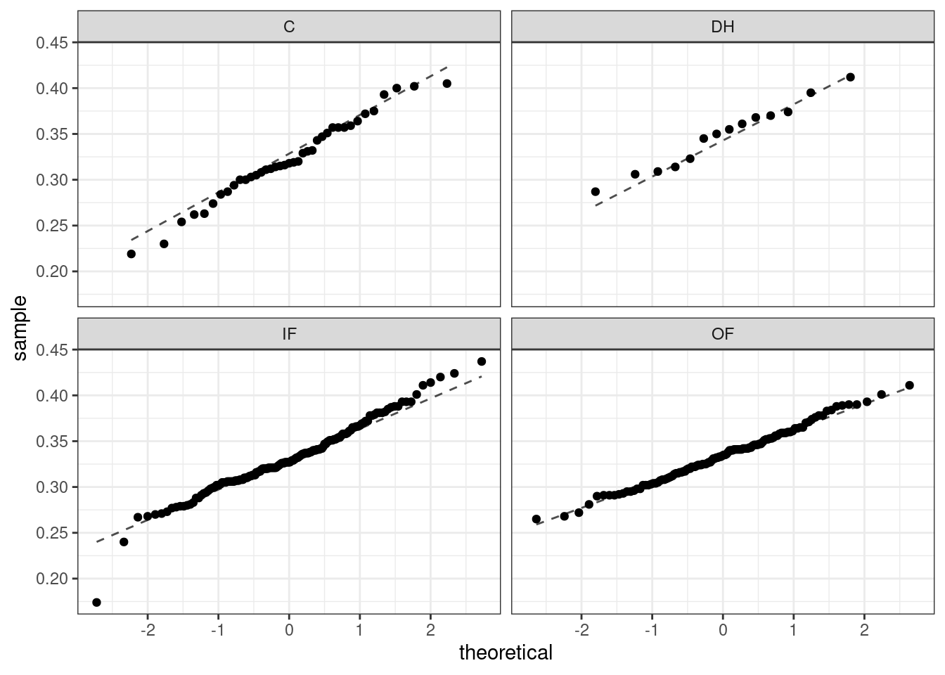
Figure 24.3: Quantile-quantile plot for two-sample test of means.
Constant variance
The last assumption is that the variance in the groups is about equal from one group to the next. This assumption can be checked by examining a side-by-side box plot of the outcomes across the groups which we did previously. In this case, the variability is similar in the four groups but not identical. We also see in the output offavstatsthat the standard deviation varies a bit from one group to the next. Whether these differences are from natural variation is unclear, so we should report this uncertainty of meeting this assumption when the final results are reported. The permutation test does not have this assumption and can be used as a check on the results from the ANOVA.
In summary, independence is always important to an ANOVA analysis. The normality condition is very important when the sample sizes for each group are relatively small. The constant variance condition is especially important when the sample sizes differ between groups.
Let’s write the hypotheses again.
\(H_0\): The average on-base percentage is equal across the four positions.
\(H_A\): The average on-base percentage varies across some (or all) groups.
The test statistic is the ratio of the between means variance and the pooled within group variance.
##              Df Sum Sq  Mean Sq F value Pr(>F)
## position      3 0.0076 0.002519   1.994  0.115
## Residuals   323 0.4080 0.001263
The table contains all the information we need. It has the degrees of freedom, mean squared errors, test statistic, and p-value. The test statistic is 1.994, \(\frac{0.002519}{0.001263}=1.994\). The p-value is larger than 0.05, indicating the evidence is not strong enough to reject the null hypothesis at a significance level of 0.05. That is, the data do not provide strong evidence that the average on-base percentage varies by player’s primary field position.
The calculation of the p-value is
pf(1.994,3,323,lower.tail = FALSE)## [1] 0.1147443Figure 24.4 is a plot of the \(F\) distribution.
gf_dist("f",df1=3,df2=323) %>%
  gf_vline(xintercept = 1.994,color="red") %>%
  gf_theme(theme_classic()) %>%
  gf_labs(title="F distribution",x="F value")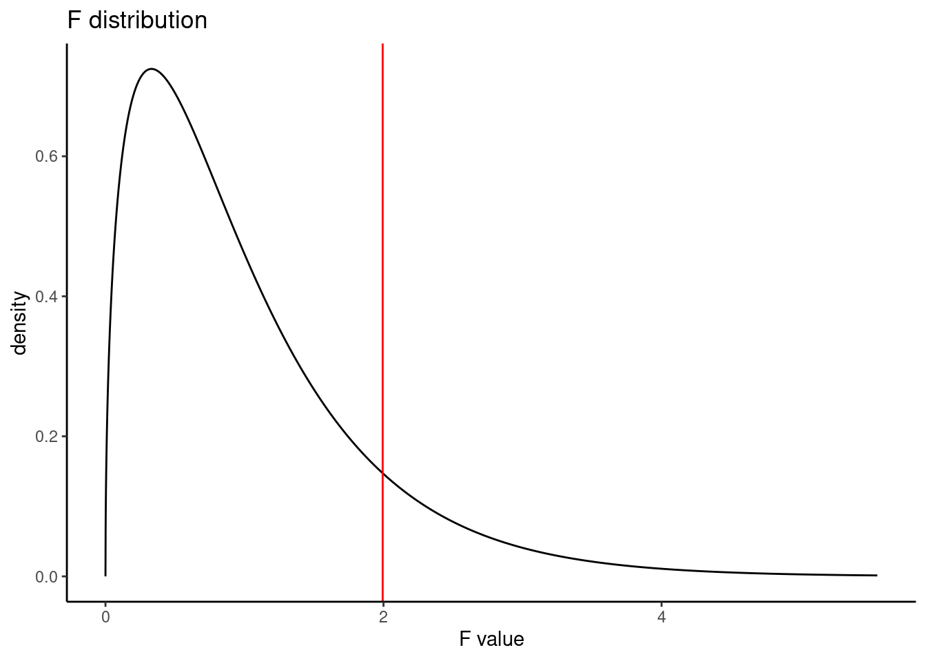
Figure 24.4: The F distribution
24.4.2.2 Permutation test
We can repeat the same analysis using a permutation test. We will first run it using a ratio of variances and then for interest as a difference in variances.
We need a way to extract the mean squared errors from the output. There is a package called broom and within it a function called tidy() that cleans up output from functions and makes them into data frames.
## # A tibble: 2 × 6
##   term         df   sumsq  meansq statistic p.value
##   <chr>     <dbl>   <dbl>   <dbl>     <dbl>   <dbl>
## 1 position      3 0.00756 0.00252      1.99   0.115
## 2 Residuals   323 0.408   0.00126     NA     NA
Let’s summarize the values in the meansq column and develop our test statistic, we could just pull the statistic but we want to be able to generate a difference test statistic as well.
## # A tibble: 1 × 1
##    stat
##   <dbl>
## 1  1.99
Now we are ready. First get our test statistic using pull().
obs<-aov(obp~position,data=mlb_obp) %>%
  tidy() %>%
  summarize(stat=meansq[1]/meansq[2]) %>%
  pull()
obs
## [1] 1.994349Let’s put our test statistic into a function to include shuffling the position variable.
f_stat <- function(x){
  aov(obp~shuffle(position),data=x) %>%
  tidy() %>%
  summarize(stat=meansq[1]/meansq[2]) %>%
  pull()
}
f_stat(mlb_obp)## [1] 0.4160649Next we run the randomization test using the do() function. There is an easier way to do all of this work with the purrr package but we will continue with the work we have started.
That was slow in executing because we are using tidyverse functions that are slow.
Figure 24.5 is a plot of the sampling distribution from the randomization test.
results %>%
  gf_dhistogram(~result,fill="cyan",color="black") %>%
  gf_dist("f",df1=3,df2=323,color="darkblue") %>%
  gf_vline(xintercept = 1.994,color="red") %>%
  gf_theme(theme_classic()) %>%
  gf_labs(title="Randomization test sampling distribution",
          subtitle="F distribution is overlayed in blue",
          x="Test statistic")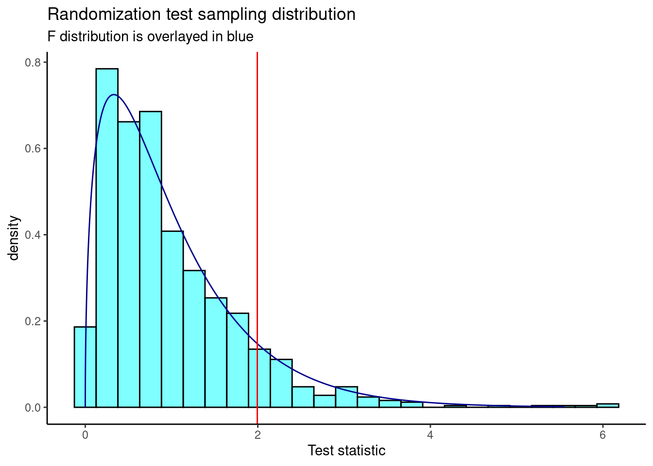
Figure 24.5: The sampling distribution of the randomization test statistic.
The p-value is
prop1(~(result>=obs),results)## prop_TRUE
## 0.0959041This is a similar p-value from the ANOVA output.
Now let’s repeat the analysis but use the difference in variance as our test statistic.
f_stat2 <- function(x){
  aov(obp~shuffle(position),data=x) %>%
  tidy() %>%
  summarize(stat=meansq[1]-meansq[2]) %>%
  pull(stat)
}Figure 24.6 is the plot of the sampling distribution of the difference in variance.
results %>%
  gf_dhistogram(~result,fill="cyan",color="black") %>%
  gf_vline(xintercept = 0.001255972,color="red") %>%
  gf_theme(theme_classic()) %>%
  gf_labs(title="Randomization test sampling distribution",
          subtitle="Test statistic is the difference in variances",
          x="Test statistic")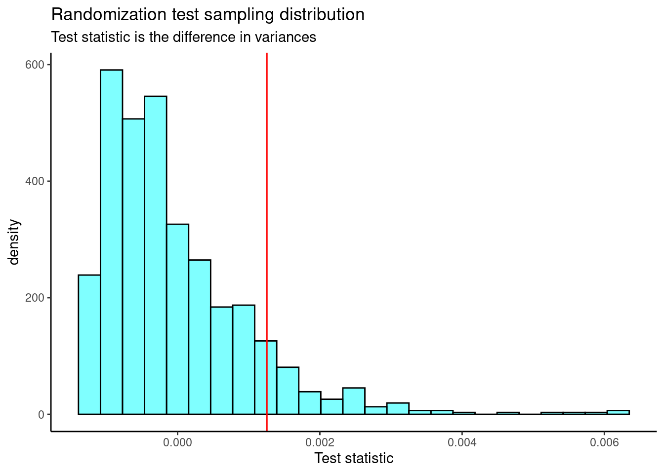
Figure 24.6: The sampling distribution of the difference in variance randomization test statistic.
We need the observed value to find a p-value.
obs<-aov(obp~position,data=mlb_obp) %>%
  tidy() %>%
  summarize(stat=meansq[1]-meansq[2]) %>%
  pull(stat)
obs
## [1] 0.001255972The p-value is
prop1(~(result>=obs),results)## prop_TRUE
## 0.0959041Again a similar p-value.
If we reject in the ANOVA test, we know there is a difference in at least one mean but we don’t know which ones. How would you approach answering that question, which means are different?
24.5 Homework Problems
- Golf balls
Repeat the analysis of the golf ball problem from earlier in the book.
- Load the data and tally the data into a table. The data is in
golf_balls.csv.
- Using the function
chisq.test(), conduct a hypothesis test of equally likely distribution of balls. You may have to read the help menu.
- Repeat part b. but assume balls with the numbers 1 and 2 occur 30% of the time and balls with 3 and 4 occur 20%.
- Bootstrap hypothesis testing
Repeat the analysis of the MLB data from the reading but this time generate a bootstrap distribution of the \(F\) statistic.
- Test of variance
We have not performed a test of variance so we will create our own.
Using the MLB from the reading, subset on
IFandOF.Create a side-by-side boxplot.
The hypotheses are:
\(H_0\): \(\sigma^2_{IF}=\sigma^2_{OF}\). There is no difference in the variance of on base percentage for infielders and outfielders.
\(H_A\): \(\sigma^2_{IF}\neq \sigma^2_{OF}\). There is a difference in variances.
- Use the differences in sample standard deviations as your test statistic. Using a permutation test, find the p-value and discuss your decision.
- Create a bootstrap distribution of the differences in sample standard deviations, and report a 95% confidence interval. Compare with part d.