22 Confidence Intervals
22.1 Objectives
- Using asymptotic methods based on the normal distribution, construct and interpret a confidence interval for an unknown parameter.
- Describe the relationships between confidence intervals, confidence level, and sample size.
- For proportions, be able to calculate the three different approaches for confidence intervals using
R.
22.2 Confidence interval
A point estimate provides a single plausible value for a parameter. However, a point estimate is rarely perfect; usually there is some error in the estimate. In addition to supplying a point estimate of a parameter, a next logical step would be to provide a plausible range of values for the parameter.
22.2.1 Capturing the population parameter
A plausible range of values for the population parameter is called a confidence interval. Using only a point estimate is like fishing in a murky lake with a spear, and using a confidence interval is like fishing with a net. We can throw a spear where we saw a fish, but we will probably miss. On the other hand, if we toss a net in that area, we have a good chance of catching the fish.
If we report a point estimate, we probably will not hit the exact population parameter. On the other hand, if we report a range of plausible values – a confidence interval – we have a good shot at capturing the parameter.
Exercise: If we want to be very certain we capture the population parameter, should we use a wider interval or a smaller interval?86
22.2.2 Constructing a confidence interval
A point estimate is our best guess for the value of the parameter, so it makes sense to build the confidence interval around that value. The standard error, which is a measure of the uncertainty associated with the point estimate, provides a guide for how large we should make the confidence interval.
Generally, what you should know about building confidence intervals is laid out in the following steps:
Identify the parameter you would like to estimate (for example, \(\mu\)).
Identify a good estimate for that parameter (sample mean, \(\bar{X}\)).
Determine the distribution of your estimate or a function of your estimate.
Use this distribution to obtain a range of feasible values (confidence interval) for the parameter. (For example if \(\mu\) is the parameter of interest and we are using the CLT, then \(\frac{\bar{X}-\mu}{\sigma/\sqrt{n}}\sim \textsf{Norm}(0,1)\). We can solve the equation for \(\mu\) to find a reasonable range of feasible values.)
Let’s do an example to solidify these ideas.
Constructing a 95% confidence interval for the mean
When the sampling distribution of a point estimate can reasonably be modeled as normal, the point estimate we observe will be within 1.96 standard errors of the true value of interest about 95% of the time. Thus, a 95% confidence interval for such a point estimate can be constructed:
\[ \hat{\theta} \pm\ 1.96 \times SE_{\hat{\theta}}\] Where \(\hat{\theta}\) is our estimate of the parameter and \(SE_{\hat{\theta}}\) is the standard error of that estimate.
We can be 95% confident this interval captures the true value. The 1.96 can be found using the qnorm() function. If we want .95 in the middle, that leaves 0.025 in each tail. Thus we use .975 in the qnorm() function.
qnorm(.975)## [1] 1.959964Exercise:
Compute the area between -1.96 and 1.96 for a normal distribution with mean 0 and standard deviation 1.
## [1] 0.9500042In mathematical terms, the derivation of this confidence is as follows:
Let \(X_1,X_2,...,X_n\) be an iid sequence of random variables, each with mean \(\mu\) and standard deviation \(\sigma\). The central limit theorem tells us that \[ \frac{\bar{X}-\mu}{\sigma/\sqrt{n}}\overset{approx}{\sim}\textsf{Norm}(0,1) \]
If the significance level is \(0\leq \alpha \leq 1\), then the confidence level is \(1-\alpha\). Yes \(\alpha\) is the same as the significance level in hypothesis testing. Thus \[ \mbox{P}\left(-z_{\alpha/2}\leq {\bar{X}-\mu\over \sigma/\sqrt{n}} \leq z_{\alpha/2}\right)=1-\alpha \]
where \(z_{\alpha/2}\) is such that \(\mbox{P}(Z\geq z_{\alpha/2})=\alpha/2\), where \(Z\sim \textsf{Norm}(0,1)\), see Figure 22.1.
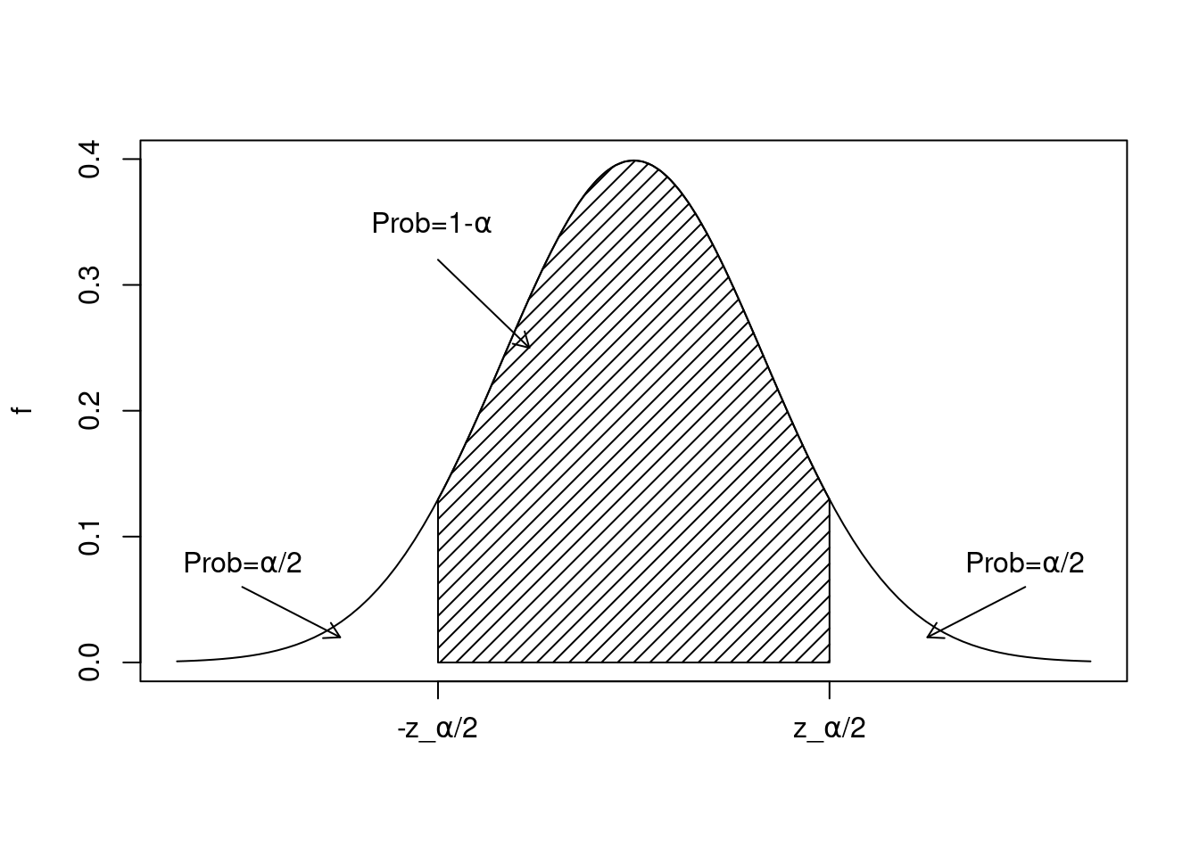
Figure 22.1: The pdf of a standard normal distribution showing idea of how to develop a confidence interval.
So, we know that \((1-\alpha)*100\%\) of the time, \({\bar{X}-\mu\over \sigma/\sqrt{n}}\) will be between \(-z_{\alpha/2}\) and \(z_{\alpha/2}\).
By rearranging the expression above and solving for \(\mu\), we get: \[ \mbox{P}\left(\bar{X}-z_{\alpha/2}{\sigma\over\sqrt{n}}\leq \mu \leq \bar{X}+z_{\alpha/2}{\sigma\over\sqrt{n}}\right)=1-\alpha \]
Be careful with the interpretation of this expression. As a reminder \(\bar{X}\) is the random variable here. The population mean, \(\mu\), is NOT a variable. It is an unknown parameter. Thus, the above expression is NOT a probabilistic statement about \(\mu\), but rather about the random variable \(\bar{X}\).
Nonetheless, the above expression gives us a nice interval for “reasonable” values of \(\mu\) given a particular sample.
A \((1-\alpha)*100\%\) confidence interval for the mean is given by: \[ \mu\in\left(\bar{x}\pm z_{\alpha/2}{\sigma\over\sqrt{n}}\right) \]
Notice in this equation we are using the lower case \(\bar{x}\), the sample mean, and thus nothing is random in the interval. Thus we will not use probabilistic statements about confidence intervals when we calculate numerical values from data for the upper and/or lower limits.
In most applications, the most common value of \(\alpha\) is 0.05. In that case, to construct a 95% confidence interval, we would need to find \(z_{0.025}\) which can be found quickly with qnorm():
qnorm(1-0.05/2)## [1] 1.959964
qnorm(.975)## [1] 1.95996422.2.2.1 Unknown Variance
When inferring about the population mean, we usually will have to estimate the underlying standard deviation as well. This introduces an extra level of uncertainty. We found that while \({\bar{X}-\mu\over\sigma/\sqrt{n}}\) has an approximate normal distribution, \({\bar{X}-\mu\over S/\sqrt{n}}\) follows the \(t\)-distribution with \(n-1\) degrees of freedom. This adds the additional assumption that the parent population, the distribution of \(X\), must be normal.
Thus, when \(\sigma\) is unknown, a \((1-\alpha)*100\%\) confidence interval for the mean is given by: \[ \mu\in\left(\bar{x}\pm t_{\alpha/2,n-1}{s\over\sqrt{n}}\right) \]
Similar to the case above, \(t_{\alpha/2,n-1}\) can be found using the qt() function in R.
In practice, if \(X\) is close to symmetrical and unimodal, we can relax the assumption of normality. Always look at your sample data. Outliers or skewness can be causes of concern. You can always run other methods that don’t require the assumption of normality and compare results.
For large sample sizes, the choice of using the normal distribution or the \(t\) distribution is irrelevant since they are close to each other. The \(t\) distribution requires you to use the degrees of freedom so be careful.
22.2.3 Body Temperature Example
Example:
Find a 95% confidence interval for the body temperature data from last lesson.
We need the mean, standard deviation, and sample size from this data. The following R code calculates the confidence interval, make sure you can follow the code.
temperature %>%
  favstats(~temperature,data=.) %>%
  select(mean,sd,n) %>%
  summarise(lower_bound=mean-qt(0.975,129)*sd/sqrt(n),
            upper_bound=mean+qt(0.975,129)*sd/sqrt(n))
## lower_bound upper_bound
## 1 98.122 98.37646The 95% confidence interval for \(\mu\) is \((98.12,98.38)\). We are 95% confident that \(\mu\), the average human body temperature, is in this interval. Alternatively and equally relevant, we could say that 95% of similarly constructed intervals will contain the true mean, \(\mu\). It is important to understand the use of the word confident and not the word probability.
There is a link between hypothesis testing and confidence intervals. Remember when we used this data in a hypothesis test, the null hypothesis was \(H_0\): The average body temperature is 98.6 \(\mu = 98.6\). This null hypothesized value is not in the interval, so we could reject the null hypothesis with this confidence interval.
We could also use R to find the confidence interval and conduct the hypothesis test. Read about the function t_test() in the help menu to determine why we used the mu option.
t_test(~temperature,data=temperature,mu=98.6)##
## One Sample t-test
##
## data: temperature
## t = -5.4548, df = 129, p-value = 2.411e-07
## alternative hypothesis: true mean is not equal to 98.6
## 95 percent confidence interval:
## 98.12200 98.37646
## sample estimates:
## mean of x
## 98.24923Or if you just want the interval:
##   mean of x  lower    upper level
## 1  98.24923 98.122 98.37646  0.95
In reviewing the hypothesis test for a single mean, you can see how this confidence interval was formed by inverting the test statistic. As a reminder, the following equation inverts the test statistic.
\[ \mbox{P}\left(\bar{X}-z_{\alpha/2}{\sigma\over\sqrt{n}}\leq \mu \leq \bar{X}+z_{\alpha/2}{\sigma\over\sqrt{n}}\right)=1-\alpha \]
22.2.4 One-sided Intervals
If you remember the hypothesis test for temperature in the central limit theorem lesson, you may be crying foul. That was a one-sided hypothesis test and we just conducted a two-sided test. So far, we have discussed only “two-sided” intervals. These intervals have an upper and lower bound. Typically, \(\alpha\) is apportioned equally between the two tails. (Thus, we look for \(z_{\alpha/2}\).)
In “one-sided” intervals, we only bound the interval on one side. We construct one-sided intervals when we are concerned with whether a parameter exceeds or stays below some threshold. Building a one-sided interval is similar to building two-sided intervals, except rather than dividing \(\alpha\) into two, you simply apportion all of \(\alpha\) to the relevant side. The difficult part is to determine if we need an upper bound or lower bound.
For the body temperature study, the alternative hypothesis was that the mean was less than 98.6. In our confidence interval, we want to find the largest value the mean could be and thus we want the upper bound. We are trying to reject the hypothesis by showing an alternative that is smaller than the null hypothesized value. Finding the lower limit does not help us since the confidence interval indicates an interval that starts at the lower value and is unbounded above. Let’s just make up some numbers; suppose the lower confidence bound is 97.5. All we know is the true average temperature is this value or greater. This is not helpful. However, if we find an upper confidence bound and the value is 98.1, we know the true average temperature is most likely no larger than this value. This is much more helpful.
Repeating the analysis with this in mind.
temperature %>%
  favstats(~temperature,data=.) %>%
  select(mean,sd,n) %>%
  summarise(upper_bound=mean+qt(0.95,129)*sd/sqrt(n))
## upper_bound
## 1 98.35577## mean of x lower upper level
## 1 98.24923 -Inf 98.35577 0.95Notice the upper bound in the one-sided interval is smaller than the upper bound in the two-sided interval since all 0.05 is going into the upper tail.
22.3 Confidence intervals for two proportions
In hypothesis testing we had several examples of two proportions. We tested these problems with a permutation test or using a hypergeometric. In our chapters and homework, we have not presented the hypothesis test for two proportions using the asymptotic normal distribution, the central limit theorem. So in this chapter we will present three methods of answering our research question, a permutation test, a hypothesis test using the normal distribution, and a confidence interval.
Earlier this book, in fact in the first chapter, we encountered an experiment that examined whether implanting a stent in the brain of a patient at risk for a stroke helps reduce the risk of a stroke. The results from the first 30 days of this study, which included 451 patients, are summarized in the R code below. These results are surprising! The point estimate suggests that patients who received stents may have a higher risk of stroke: \(p_{trmt} - p_{control} = 0.090\).
stent <- read_csv("data/stent_study.csv")
tally(~group+outcome30,data=stent,margins = TRUE)## outcome30
## group no_event stroke Total
## control 214 13 227
## trmt 191 33 224
## Total 405 46 451
tally(outcome30~group,data=stent,margins = TRUE,format="proportion")## group
## outcome30 control trmt
## no_event 0.94273128 0.85267857
## stroke 0.05726872 0.14732143
## Total 1.00000000 1.00000000
obs<-diffprop(outcome30~group,data=stent)
obs
## diffprop
## -0.09005271Notice that because R uses the variables by names in alphabetic order we have \(p_{control} - p_{trmt} = - 0.090\). This is not a problem. We could fix this by changing the variables to factors.
22.3.1 Permutation test for two proportions
We start with the null hypothesis which is two-sided since we don’t know if the treatment is harmful or beneficial.
\(H_0\): The treatment and outcome are independent. \(p_{control} - p_{trmt} = 0\) or \(p_{control} = p_{trmt}\).
\(H_A\): The treatment and outcome are dependent \(p_{control} \neq p_{trmt}\).
We will use \(\alpha = 0.05\).
The test statistic is the difference in proportions of patients with stroke in the control and treatment groups.
obs<-diffprop(outcome30~group,data=stent)
obs
## diffprop
## -0.09005271To calculate the p-value, we will shuffle the treatment and control labels because under the null hypothesis, there is no difference.
Figure 22.2 a visual summary of the distribution of the test statistics generated under the null hypothesis, the sampling distribution.
results %>%
  gf_dhistogram(~diffprop,fill="cyan",color="black") %>%
  gf_vline(xintercept =obs ) %>%
  gf_theme(theme_classic()) %>%
  gf_labs(title="Sampling distribution of randomization test",
          x="Difference in proportions",y="")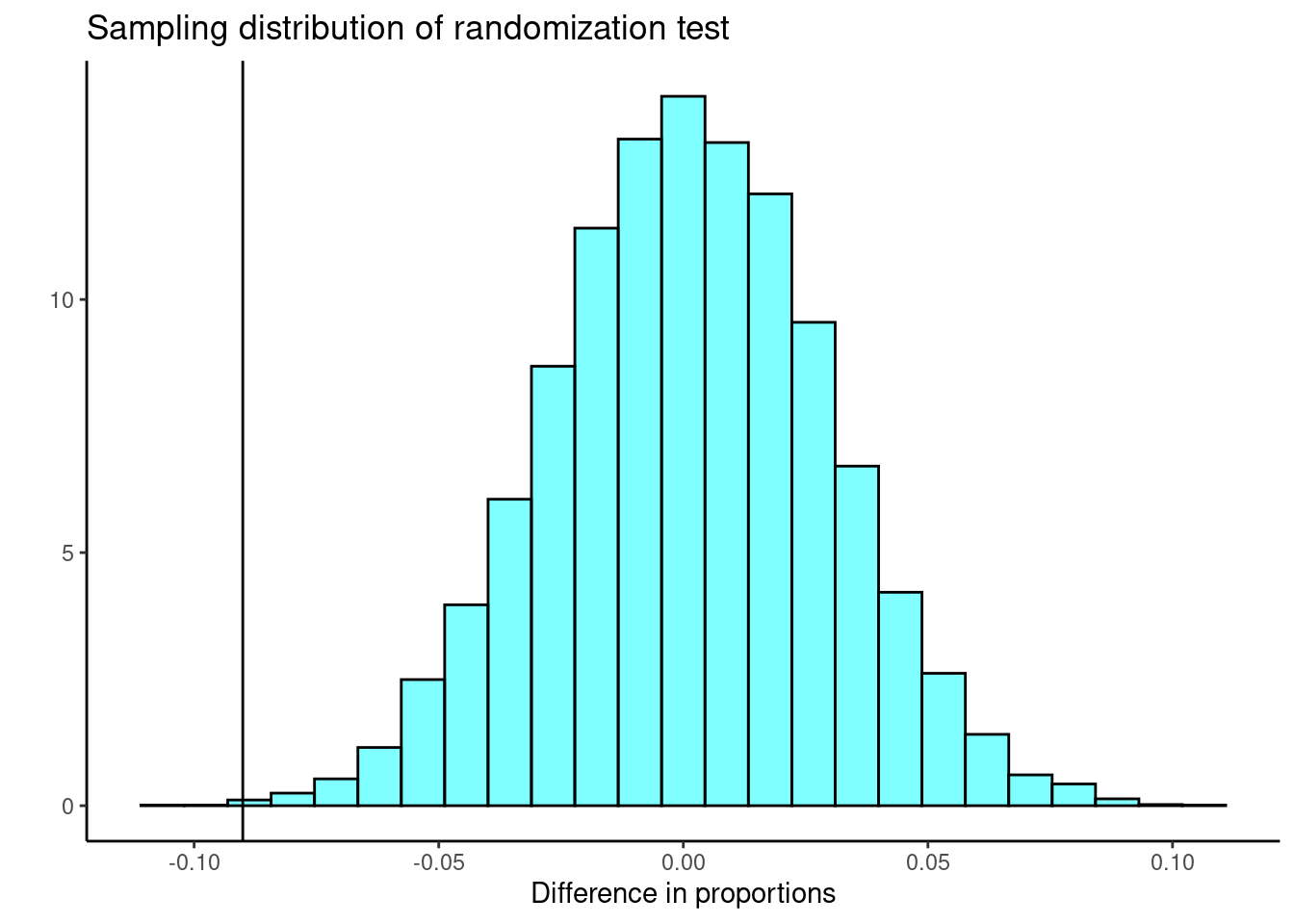
Figure 22.2: Sampling distribution of the difference in proportions.
We next calculate the p-value. We will calculate it as if it were a one-sided test and then double the result to account for the fact that we would reject with a similar value in the opposite tail. Note that the prop1() includes the observed value in the calculation of the p-value.
2*prop1(~(diffprop<=obs),data=results)## prop_TRUE
## 0.00259974Based on the data, if there were no difference between the treatment and control groups, the probability of the observed differences in proportion of strokes being - 0.09 or more extreme is 0.0026. This is too unlikely, so we reject that there is no difference between control and stroke groups.
22.3.2 Hypothesis test for two proportions using normal model
We must check two conditions before applying the normal model to a generic test of \(\hat{p}_1 - \hat{p}_2\). First, the sampling distribution for each sample proportion must be nearly normal, and secondly, the samples must be independent. Under these two conditions, the sampling distribution of \(\hat{p}_1 - \hat{p}_2\) may be well approximated using the normal model.
The hypotheses are the same as above.
22.3.2.1 Conditions for the sampling distribution of \(\hat{p}_1 - \hat{p}_2\) to be normal
The difference \(\hat{p}_1 - \hat{p}_2\) tends to follow a normal model when
- each proportion separately follows a normal model, and
- the two samples are independent of each other
22.3.2.2 Standard error
For our research question the conditions must be verified. Because each group is a simple random sample from less than 10% of the population, the observations are independent, both within the samples and between the samples. The success-failure condition also holds for each sample, at least 10 in each cell is the easiest way to think about it. Because all conditions are met, the normal model can be used for the point estimate of the difference in proportion of strokes
\[p_{control} - p_{trmt} = 0.05726872 - 0.14732143 = - 0.090\] The standard error of the difference in sample proportions is \[ SE_{\hat{p}_1 - \hat{p}_2} = \sqrt{SE_{\hat{p}_1}^2 + SE_{\hat{p}_2}^2}\] \[ = \sqrt{\frac{p_1(1-p_1)}{n_1} + \frac{p_2(1-p_2)}{n_2}}\] where \(p_1\) and \(p_2\) represent the population proportions, and \(n_1\) and \(n_2\) represent the sample sizes.
The calculation of the standard error for our problem must be done carefully. Remember in hypothesis testing, we assume the null hypothesis is true; this means the proportions of strokes must be the same.
\[SE = \sqrt{\frac{p(1-p)}{n_{control}} + \frac{p(1-p)}{n_{trmt}}}\] We don’t know the exposure rate, \(p\), but we can obtain a good estimate of it by pooling the results of both samples: \[\hat{p} = \frac{\text{# of successes}}{\text{# of cases}} = \frac{13 + 33}{451} = 0.102\] This is called the pooled estimate of the sample proportion, and we use it to compute the standard error when the null hypothesis is that \(p_{control} = p_{trmt}\).
\[SE \approx \sqrt{\frac{\hat{p}(1-\hat{p})}{n_{control}} + \frac{\hat{p}(1-\hat{p})}{n_{trmt}}}\]
\[SE \approx \sqrt{\frac{0.102(1-0.102)}{227} + \frac{0.102(1-0.102)}{224}} = 0.0285\]
The test statistic is \[Z = \frac{\text{point estimate} - \text{null value}}{SE} = \frac{-.09 - 0}{0.0285} = - 3.16 \]
The p-value is
2*pnorm(-3.16)## [1] 0.001577691Which is close to what we got with permutation test. This should not surprise us as the sampling distribution under the permutation test looked normal.
Figure 22.3 plots the empirical sampling distribution from the permutation test again with a normal density curve overlayed.
results %>%
  gf_dhistogram(~diffprop,fill="cyan",color="black") %>%
  gf_vline(xintercept =obs ) %>%
  gf_dist("norm",sd=0.0285,color="red") %>%
  gf_theme(theme_classic()) %>%
  gf_labs(title="Sampling distribution of randomization test",
          subtitle="Reference normal distribution in red",
          x="Difference in proportions")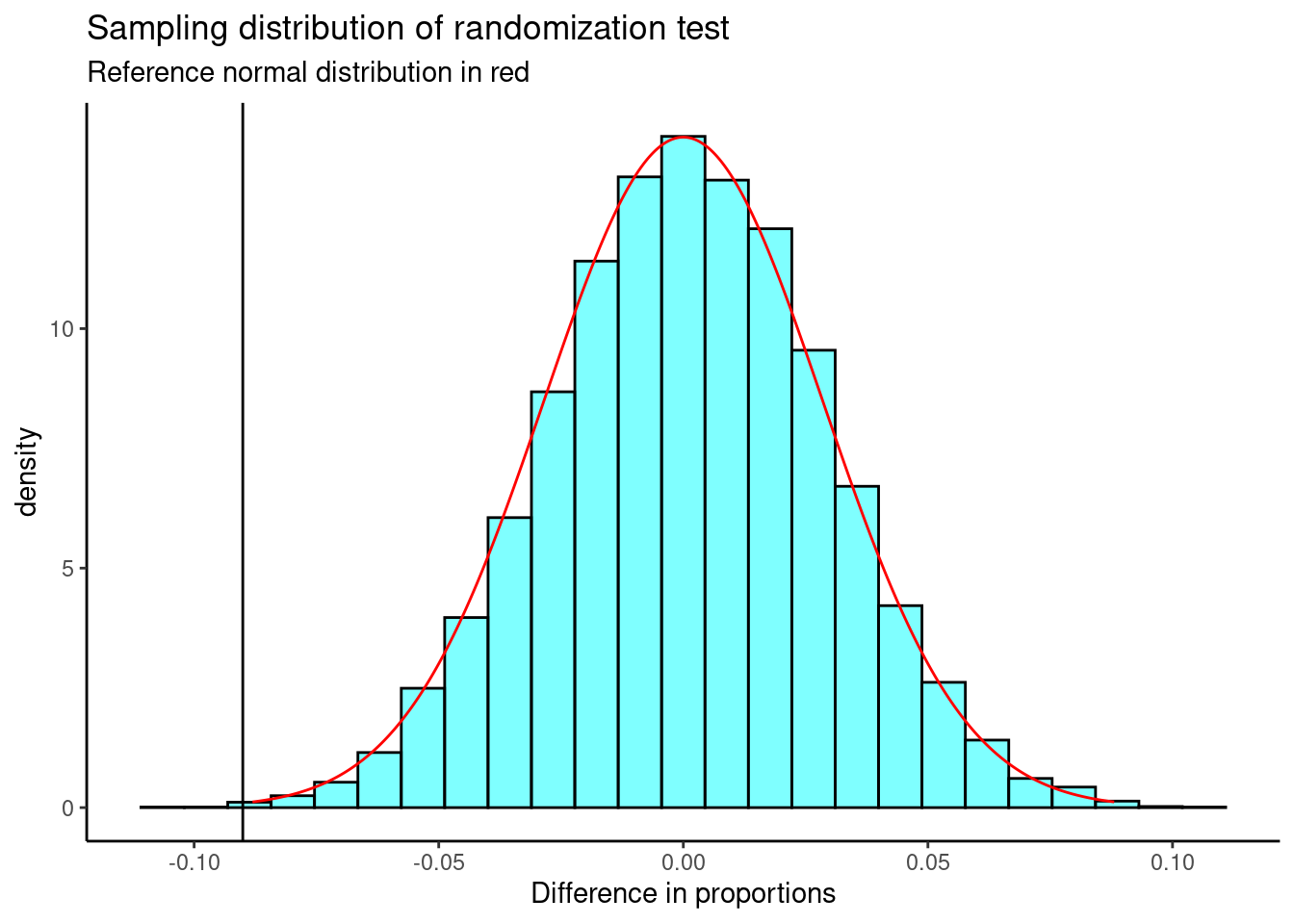
Figure 22.3: The sampling distribution of the randomization test with a normal distribution plotted in red.
22.3.3 Confidence interval for two proportions using normal model
The conditions for applying the normal model have already been verified, so we can proceed to the construction of the confidence interval. Remember the form of the confidence interval is
\[\text{point estimate} \ \pm\ z^{\star}SE\]
Our point estimate is -0.09. The standard error is different since we can’t assume the proportion of strokes are equal. We will estimate the standard error from
\[SE = \sqrt{\frac{p_{control}(1-p_{control})}{n_{control}} + \frac{p_{trmt}(1-p_{trmt})}{n_{trmt}}}\]
\[SE \approx \sqrt{\frac{0.057(1-0.057)}{227} + \frac{0.15(1-0.15)}{224}} = 0.0284\]
It is close to the pooled value because of the nearly equal sample sizes.
The critical value is found from the normal quantile.
qnorm(.975)## [1] 1.959964The 95% confidence interval is
\[ - 0.09 \ \pm\ 1.96 \times 0.0284 \quad \to \quad (-0.146,- 0.034)\] We are 95% confident that the difference in proportions of strokes in the control and treatment groups is between -0.146 and -0.034. Since this does not include zero, we are confident they are different. This supports the hypothesis tests. This confidence interval is not an accurate method for smaller samples sizes. This is because the actual coverage rate, the percentage of intervals that contain the true population parameter, will not be the nomial coverage rate. This means it is not true that 95% of similarly constructed 95% confidence intervals will contain the true parameter. This because the pooled estimate of the standard error is not accurate for small sample sizes. For the example above, the sample sizes are large and the performance of the method should be adequate.
Of course, R has a built in function to calculate the hypothesis test and confidence interval for two proportions.
prop_test(outcome30~group,data=stent)##
## 2-sample test for equality of proportions with continuity correction
##
## data: tally(outcome30 ~ group)
## X-squared = 9.0233, df = 1, p-value = 0.002666
## alternative hypothesis: two.sided
## 95 percent confidence interval:
## 0.03022922 0.14987619
## sample estimates:
## prop 1 prop 2
## 0.9427313 0.8526786The p-value is a little different from the one we calculated and closer to the randomization test, which is an approximation of the exact permutation test, because a correction factor was applied. Read online about this correction to learn more. We run the code below with the correction factor off and get the same p-value as we calculated above. The confidence interval is a little different because the function used no stroke as its success event, but since zero is not in the interval, we get the same conclusion.
prop_test(outcome30~group,data=stent,correct=FALSE)##
## 2-sample test for equality of proportions without continuity
## correction
##
## data: tally(outcome30 ~ group)
## X-squared = 9.9823, df = 1, p-value = 0.001581
## alternative hypothesis: two.sided
## 95 percent confidence interval:
## 0.03466401 0.14544140
## sample estimates:
## prop 1 prop 2
## 0.9427313 0.8526786Essentially, confidence intervals and hypothesis tests serve similar purposes, but answer slightly different questions. A confidence interval gives you a range of feasible values of a parameter given a particular sample. A hypothesis test tells you whether a specific value is feasible given a sample. Sometimes you can informally conduct a hypothesis test simply by building an interval and observing whether the hypothesized value is contained in the interval. The disadvantage to this approach is that it does not yield a specific \(p\)-value. The disadvantage of the hypothesis test is that it does not give a range of values for the test statistic.
As with hypothesis tests, confidence intervals are imperfect. About 1-in-20 properly constructed 95% confidence intervals will fail to capture the parameter of interest. This is a similar idea to our Type 1 error.
22.4 Changing the confidence level
Suppose we want to consider confidence intervals where the confidence level is somewhat higher than 95%; perhaps we would like a confidence level of 99%. Think back to the analogy about trying to catch a fish: if we want to be more sure that we will catch the fish, we should use a wider net. To create a 99% confidence level, we must also widen our 95% interval. On the other hand, if we want an interval with lower confidence, such as 90%, we could make our original 95% interval slightly slimmer.
The 95% confidence interval structure provides guidance in how to make intervals with new confidence levels. Below is a general 95% confidence interval for a point estimate that comes from a nearly normal distribution:
\[\text{point estimate}\ \pm\ 1.96\times SE \]
There are three components to this interval: the point estimate, “1.96,” and the standard error. The choice of \(1.96\times SE\), which is also called margin of error, was based on capturing 95% of the data since the estimate is within 1.96 standard errors of the true value about 95% of the time. The choice of 1.96 corresponds to a 95% confidence level.
Exercise: If \(X\) is a normally distributed random variable, how often will \(X\) be within 2.58 standard deviations of the mean?87
To create a 99% confidence interval, change 1.96 in the 95% confidence interval formula to be \(2.58\).
The normal approximation is crucial to the precision of these confidence intervals. We will learn a method called the bootstrap that will allow us to find confidence intervals without the assumption of normality.
22.5 Interpreting confidence intervals
A careful eye might have observed the somewhat awkward language used to describe confidence intervals.
Correct interpretation:
We are XX% confident that the population parameter is between…
Incorrect language might try to describe the confidence interval as capturing the population parameter with a certain probability. This is one of the most common errors: while it might be useful to think of it as a probability, the confidence level only quantifies how plausible it is that the parameter is in the interval.
Another especially important consideration of confidence intervals is that they only try to capture the population parameter. Our intervals say nothing about the confidence of capturing individual observations, a proportion of the observations, or about capturing point estimates. Confidence intervals only attempt to capture population parameters.
22.6 Homework Problems
- Chronic illness
In 2013, the Pew Research Foundation reported that “45% of U.S. adults report that they live with one or more chronic conditions.”88 However, this value was based on a sample, so it may not be a perfect estimate for the population parameter of interest on its own. The study reported a standard error of about 1.2%, and a normal model may reasonably be used in this setting.
- Create a 95% confidence interval for the proportion of U.S. adults who live with one or more chronic conditions. Also interpret the confidence interval in the context of the study.
- Create a 99% confidence interval for the proportion of U.S. adults who live with one or more chronic conditions. Also interpret the confidence interval in the context of the study.
- Identify each of the following statements as true or false. Provide an explanation to justify each of your answers.
- We can say with certainty that the confidence interval from part a contains the true percentage of U.S. adults who suffer from a chronic illness.
- If we repeated this study 1,000 times and constructed a 95% confidence interval for each study, then approximately 950 of those confidence intervals would contain the true fraction of U.S. adults who suffer from chronic illnesses.
- The poll provides statistically significant evidence (at the \(\alpha = 0.05\) level) that the percentage of U.S. adults who suffer from chronic illnesses is not 50%.
- Since the standard error is 1.2%, only 1.2% of people in the study communicated uncertainty about their answer.
- Suppose the researchers had formed a one-sided hypothesis, they believed that the true proportion is less than 50%. We could find an equivalent one-sided 95% confidence interval by taking the upper bound of our two-sided 95% confidence interval.
- Vegetarian college students
Suppose that 8% of college students are vegetarians. Determine if the following statements are true or false, and explain your reasoning.
- The distribution of the sample proportions of vegetarians in random samples of size 60 is approximately normal since \(n \ge 30\).
- The distribution of the sample proportions of vegetarian college students in random samples of size 50 is right skewed.
- A random sample of 125 college students where 12% are vegetarians would be considered unusual.
- A random sample of 250 college students where 12% are vegetarians would be considered unusual.
- The standard error would be reduced by one-half if we increased the sample size from 125 to~250.
- A 99% confidence will be wider than a 95% because to have a higher confidence level requires a wider interval.
- Orange tabbies
Suppose that 90% of orange tabby cats are male. Determine if the following statements are true or false, and explain your reasoning.
a. The distribution of sample proportions of random samples of size 30 is left skewed.
b. Using a sample size that is 4 times as large will reduce the standard error of the sample proportion by one-half.
c. The distribution of sample proportions of random samples of size 140 is approximately normal.
- Working backwards
A 90% confidence interval for a population mean is (65,77). The population distribution is approximately normal and the population standard deviation is unknown. This confidence interval is based on a simple random sample of 25 observations. Calculate the sample mean, the margin of error, and the sample standard deviation.
- Find the p-value
An independent random sample is selected from an approximately normal population with an unknown standard deviation. Find the p-value for the given set of hypotheses and \(T\) test statistic. Also determine if the null hypothesis would be rejected at \(\alpha = 0.05\).
-
\(H_{A}: \mu > \mu_{0}\), \(n = 11\), \(T = 1.91\)
-
\(H_{A}: \mu < \mu_{0}\), \(n = 17\), \(T = - 3.45\)
-
\(H_{A}: \mu \ne \mu_{0}\), \(n = 7\), \(T = 0.83\)
- \(H_{A}: \mu > \mu_{0}\), \(n = 28\), \(T = 2.13\)
- Sleep habits of New Yorkers
New York is known as “the city that never sleeps.” A random sample of 25 New Yorkers were asked how much sleep they get per night. Statistical summaries of these data are shown below. Do these data provide strong evidence that New Yorkers sleep less than 8 hours a night on average?
\[ \begin{array}{ccccc} & & &\\ \hline n & \bar{x} & s & min & max \\ \hline 25 & 7.73 & 0.77 & 6.17 & 9.78 \\ \hline \end{array} \]
- Write the hypotheses in symbols and in words.
- Check conditions, then calculate the test statistic, \(T\), and the associated degrees of freedom.
- Find and interpret the p-value in this context.
- What is the conclusion of the hypothesis test?
- Construct a 95% confidence interval that corresponded to this hypothesis test, would you expect 8 hours to be in the interval?
- Vegetarian college students II
From problem 2 part c, suppose that it has been reported that 8% of college students are vegetarians. We think USAFA is not typical because of their fitness and health awareness, we think there are more vegetarians. We collect a random sample of 125 cadets and find 12% claimed they are vegetarians. Is there enough evidence to claim that USAFA cadets are different?
- Use
binom.test()to conduct the hypothesis test and find a confidence interval. - Use
prop.test()withcorrect=FALSEto conduct the hypothesis test and find a confidence interval. - Use
prop.test()withcorrect=TRUEto conduct the hypothesis test and find a confidence interval. - Which test should you use?